RTN-125

Photometric Transformation Relations for the LSST Data Preview 2#

Abstract

This technical note provides photometric transformation relations between the NSF-DOE Vera C. Rubin Observatory’s Data Preview 2 (DP2) and other photometric systems. These transformations are derived using both synthetic and empirical data and are intended to support calibration and comparison across survey systems. We present both polynomial equations and lookup-table-based methods, depending on the available data and desired accuracy. The transformations are generally valid for stars with typical spectral energy distributions (SEDs), and caution should be used when applying them to objects with strong emission lines or atypical colors.

DOI: 10.71929/rubin/3399546

0. General Overview#

The transformations described in this note were obtained by cross‑matching photometric data from external surveys with the Rubin LSST DP2 data [NSF-DOE Vera C. Rubin Observatory, 2026, Vera C. Rubin Observatory Team, 2026]. Here, we provide a high‑level summary of the resulting transformation relations for converting to and from the DP2 photometric system.

This note is intended to remain a living document. As additional photometric systems are incorporated or existing DP2 transformations updated, new material will be added accordingly.

Note

Transformations between the DP1 photometric system and several external systems are available in RTN-099 [Porter et al., 2026]. RTN‑125 is still in active development and does not yet include DP2 transformations for all the systems provided in RTN-099. In the meantime, for those systems not already included below, users should apply the DP2→DP1 relations in Section 1.3.1 below, followed by the DP1→other‑system transformations provided in RTN‑099.

1. Polynomial Fit Transformations#

1.1. Overview#

A simple and popular method of performing photometric transformations between two photometric systems is to perform a polynomial fit between the difference in magnitudes between a filter band in one system (say, the LSSTCam \(i\) band) and another system (say, the DES \(i\) band) and one or more color indices in one of the two systems (say, the \((g-i)\) color in the DES system). These fits can be low-order (say, a first-degree polynomial) or high-order (say, a third or higher degree polynomial). They can be a single fit over the full color range, or they can be solved “piece-wise”, with breaks in the fit at one or more values of the color index. Here, a balance between simplicity and accuracy is attempted, aiming for the lowest-order fit that still gives a reasonable level of accuracy (typically with RMS’es of a few hundredths to a few tenths of a magnitude.) If higher accuracy is required – to the extent that complexity is not a major factor – use of the Lookup Table (Interpolation) Transformations in Section 2 is recommended.

1.2. Synthetic LSSTCam Transformations#

These transformations are based on synthetic magnitudes in DP2 and from other surveys/photometric systems. They are generally preferred only if no observed transformations are available for matched stars/objects in DP2 and the other survey/photometric system (e.g., like for LSST <–> TESS, in which TESS stars are all too bright and thus saturate in the LSST science observations).

Synthetic magnitudes were derived by integrating spectrophotometric spectra from the Pickles Stellar Spectra Library [Pickles, 1998] with filter passband transmission curves for LSSTCam and other photometric systems. These magnitudes were calculated using broad-band absolute magnitude definitions and processed using a Python-based fitting code to generate transformation equations. Due to the limited number of stars in the Pickles library (~100), the resulting plots are sparse but provide a consistent reference.

1.2.1 LSST <–> TESS#

Under Construction

1.3. Observed LSST DP2 Transformations#

These transformations are based on the actual observed magnitudes of stars in DP2 and from other surveys/photometric systems. They are generally preferred over transformations based on synthetic photometry.

1.3.1 LSST DP2 <–> LSST DP1#

Recall that LSST Data Preview 1 (DP1) [Vera C. Rubin Observatory Team, 2026, Vera C. Rubin Observatory Team et al., 2026] was performed with the LSST Commissioning Camera (LSSTComCam) [SLAC National Accelerator Laboratory and NSF-DOE Vera C. Rubin Observatory, 2024], which used only ITL CCDs. LSST Data Preview 2 (DP2) was performed with the LSST Main Camera (LSSTCam) [SLAC National Accelerator Laboratory and NSF-DOE Vera C. Rubin Observatory, 2025], which uses mostly e2v CCDs with a relatively small subset of ITL CCDS. During photometric calibration, the DP2 data are placed onto a standard system across the camera focal plane. The DP1 and DP2 standard systems differ slightly. Thus, to compare DP1 and DP2 magnitudes and colors most accurately, one should transform from one system to the other. Here are the relations to do that.

Conversion	Transformation Equation	RMS	Applicable Color Range	QA Plot
\(u_{LSST} \to u_{ComCam}\)	\(u_{ComCam} - u_{LSST} = -0.023 (g−i)LSST -0.010\)	0.054	\(-0.6 < (g−i)LSST \leq 2.8\)	link
\(g_{LSST} \to g_{ComCam}\)	\(g_{ComCam} - g_{LSST} = +0.012 (g−i)LSST -0.022\)	0.008	\(-0.6 < (g−i)LSST \leq 2.9\)	link
\(r_{LSST} \to r_{ComCam}\)	\(r_{ComCam} - r_{LSST} = -0.001 (g−i)LSST -0.001\)	0.006	\(-0.6 < (g−i)LSST \leq 2.9\)	link
\(i_{LSST} \to i_{ComCam}\)	\(i_{ComCam} - i_{LSST} = -0.010 (g−i)LSST +0.017\)	0.005	\(-0.6 < (g−i)LSST \leq 2.9\)	link
\(z_{LSST} \to z_{ComCam}\)	\(z_{ComCam} - z_{LSST} = -0.005 (i−z)LSST +0.002\)	0.005	\(-0.2 < (i−z)LSST \leq 0.7\)	link
\(y_{LSST} \to y_{ComCam}\)	\(y_{ComCam} - y_{LSST} = -0.007 (z−y)LSST -0.001\)	0.015	\(-0.2 < (z−y)LSST \leq 0.4\)	link

Conversion	Transformation Equation	RMS	Applicable Color Range	QA Plot
\(u_{ComCam} \to u_{LSST}\)	\(u_{LSST} - u_{ComCam} = +0.022 (g−i)ComCam +0.011\)	0.054	\(-0.6 < (g−i)ComCam \leq 2.8\)	link
\(g_{ComCam} \to g_{LSST}\)	\(g_{LSST} - g_{ComCam} = -0.012 (g−i)ComCam +0.021\)	0.008	\(-0.6 < (g−i)ComCam \leq 2.9\)	link
\(r_{ComCam} \to r_{LSST}\)	\(r_{LSST} - r_{ComCam} = +0.001 (g−i)ComCam +0.002\)	0.006	\(-0.6 < (g−i)ComCam \leq 2.9\)	link
\(i_{ComCam} \to i_{LSST}\)	\(i_{LSST} - i_{ComCam} = +0.010 (g−i)ComCam -0.017\)	0.005	\(-0.6 < (g−i)ComCam \leq 2.9\)	link
\(z_{ComCam} \to z_{LSST}\)	\(z_{LSST} - z_{ComCam} = +0.006 (i−z)ComCam -0.002\)	0.005	\(-0.2 < (i−z)ComCam \leq 0.7\)	link
\(y_{ComCam} \to y_{LSST}\)	\(y_{LSST} - y_{ComCam} = +0.036 (z−y)ComCam -0.002\)	0.015	\(-0.2 < (z−y)ComCam \leq 0.4\)	link

1.3.2 LSST DP2 <–> DES DR2#

Conversion	Transformation Equation	RMS	Applicable Color Range	QA Plot
\(g_{LSST} \to g_{des}\)	\(g_{des} - g_{LSST} = +0.011 (g−i)LSST -0.013\)	0.015	\(-1.0 < (g−i)LSST \leq 2.3\)	link
\(g_{LSST} \to g_{des}\)	\(g_{des} - g_{LSST} = -0.032 (g−i)LSST +0.080\)	0.026	\(2.3 < (g−i)LSST \leq 3.8\)	link

\(r_{LSST} \to r_{des}\)	\(r_{des} - r_{LSST} = -0.058 (g−i)LSST +0.005\)	0.008	\(-0.8 < (g−i)LSST \leq 2.0\)	link
\(r_{LSST} \to r_{des}\)	\(r_{des} - r_{LSST} = -0.122 (g−i)LSST +0.133\)	0.016	\(2.0 < (g−i)LSST \leq 3.8\)	link

\(i_{LSST} \to i_{des}\)	\(i_{des} - i_{LSST} = -0.049 (g−i)LSST +0.018\)	0.01	\(-0.8 < (g−i)LSST \leq 1.8\)	link
\(i_{LSST} \to i_{des}\)	\(i_{des} - i_{LSST} = -0.121 (g−i)LSST +0.144\)	0.012	\(1.8 < (g−i)LSST \leq 3.8\)	link

\(z_{LSST} \to z_{des}\)	\(z_{des} - z_{LSST} = -0.328 (i−z)LSST -0.002\)	0.009	\(-0.3 < (i−z)LSST \leq 0.2\)	link
\(z_{LSST} \to z_{des}\)	\(z_{des} - z_{LSST} = -0.217 (i−z)LSST -0.021\)	0.01	\(0.2 < (i−z)LSST \leq 1.3\)	link

\(y_{LSST} \to Y_{des}\)	\(Y_{des} - y_{LSST} = -0.119 (i−z)LSST +0.018\)	0.02	\(-0.6 < (i−z)LSST \leq 0.2\)	link
\(y_{LSST} \to Y_{des}\)	\(Y_{des} - y_{LSST} = -0.051 (i−z)LSST +0.007\)	0.018	\(0.2 < (i−z)LSST \leq 2.5\)	link

Conversion	Transformation Equation	RMS	Applicable Color Range	QA Plot
\(g_{des} \to g_{LSST}\)	\(g_{LSST} - g_{des} = -0.011 (g−i)des +0.014\)	0.014	\(-0.8 < (g−i)des \leq 2.3\)	link
\(g_{des} \to g_{LSST}\)	\(g_{LSST} - g_{des} = +0.020 (g−i)des -0.054\)	0.025	\(2.3 < (g−i)des \leq 4.0\)	link

\(r_{des} \to r_{LSST}\)	\(r_{LSST} - r_{des} = +0.054 (g−i)des -0.003\)	0.008	\(-0.8 < (g−i)des \leq 2.0\)	link
\(r_{des} \to r_{LSST}\)	\(r_{LSST} - r_{des} = +0.108 (g−i)des -0.116\)	0.015	\(2.0 < (g−i)des \leq 4.0\)	link

\(i_{des} \to i_{LSST}\)	\(i_{LSST} - i_{des} = +0.045 (g−i)des -0.016\)	0.009	\(-0.8 < (g−i)des \leq 1.8\)	link
\(i_{des} \to i_{LSST}\)	\(i_{LSST} - i_{des} = +0.109 (g−i)des -0.132\)	0.012	\(1.8 < (g−i)des \leq 4.0\)	link

\(z_{des} \to z_{LSST}\)	\(z_{LSST} - z_{des} = +0.319 (i−z)des -0.001\)	0.007	\(-0.3 < (i−z)des \leq 0.2\)	link
\(z_{des} \to z_{LSST}\)	\(z_{LSST} - z_{des} = +0.241 (i−z)des +0.013\)	0.008	\(0.2 < (i−z)des \leq 1.0\)	link

\(Y_{des} \to y_{LSST}\)	\(y_{LSST} - Y_{des} = +0.120 (i−z)des -0.019\)	0.019	\(-0.3 < (i−z)des \leq 0.2\)	link
\(Y_{des} \to y_{LSST}\)	\(y_{LSST} - Y_{des} = +0.056 (i−z)des -0.009\)	0.018	\(0.2 < (i−z)des \leq 1.1\)	link

1.3.3 LSST DP2 <–> PanStarrs1 DR2#

Conversion	Transformation Equation	RMS	Applicable Color Range	QA Plot
\(g_{LSST} \to g_{ps1}\)	\(g_{ps1} - g_{LSST} = -0.029 (g-i)_{LSST} -0.028\)	0.03	\(-0.7 < (g-i)_{LSST} \leq 3.7\)	link

\(r_{LSST} \to r_{ps1}\)	\(r_{ps1} - r_{LSST} = +0.000 (g-i)_{LSST} -0.002\)	0.017	\(-0.7 < (g-i)_{LSST} \leq 3.7\)	link

\(i_{LSST} \to i_{ps1}\)	\(i_{ps1} - i_{LSST} = +0.007 (g-i)_{LSST} -0.006\)	0.012	\(-0.7 < (g-i)_{LSST} \leq 3.7\)	link

\(z_{LSST} \to z_{ps1}\)	\(z_{ps1} - z_{LSST} = +0.007 (i-z)_{LSST} +0.004\)	0.012	\(-0.2 < (i-z)_{LSST} \leq 1.3\)	link

\(y_{LSST} \to y_{ps1}\)	\(y_{ps1} - y_{LSST} = +0.060 (z-y)_{LSST} -0.025\)	0.025	\(-0.5 < (z-y)_{LSST} \leq 1.0\)	link

Conversion	Transformation Equation	RMS	Applicable Color Range	QA Plot
\(g_{ps1} \to g_{LSST}\)	\(g_{LSST} - g_{ps1} = +0.028 (g-i)_{ps1} +0.031\)	0.031	\(-0.7 < (g-i)_{ps1} \leq 3.3\)	link

\(r_{ps1} \to r_{LSST}\)	\(r_{LSST} - r_{ps1} = -0.001 (g-i)_{ps1} +0.002\)	0.017	\(-0.7 < (g-i)_{ps1} \leq 3.4\)	link

\(i_{ps1} \to i_{LSST}\)	\(i_{LSST} - i_{ps1} = -0.007 (g-i)_{ps1} +0.006\)	0.012	\(-0.7 < (g-i)_{ps1} \leq 3.4\)	link

\(z_{ps1} \to z_{LSST}\)	\(z_{LSST} - z_{ps1} = -0.004 (i-z)_{ps1} -0.005\)	0.012	\(-0.3 < (i-z)_{ps1} \leq 1.0\)	link

\(y_{ps1} \to y_{LSST}\)	\(y_{LSST} - y_{ps1} = +0.013 (z-y)_{ps1} +0.015\)	0.026	\(-0.2 < (z-y)_{ps1} \leq 0.5\)	link

1.3.4 LSST DP2 <–> GAIA DR3#

Conversion	Transformation Equation	RMS	Applicable Color Range	QA Plot
\(g_{LSST} \to G_{gaia}\)	\(G_{gaia} - g_{LSST} = -0.037 (g-i)_{LSST}^2 -0.600 (g-i)_{LSST} -0.056\)	0.01	\(0.2 < (g-i)_{LSST} \leq 2.9\)	link

\(g_{LSST} \to BP_{gaia}\)	\(BP_{gaia} - g_{LSST} = +0.096 (g-i)_{LSST}^2 -0.487 (g-i)_{LSST} +0.194\)	0.037	\(0.3 < (g-i)_{LSST} \leq 3.2\)	link

\(r_{LSST} \to RP_{gaia}\)	\(RP_{gaia} - r_{LSST} = -0.267 (g-i)_{LSST}^2 +0.242 (g-i)_{LSST} -0.563\)	0.043	\(0.3 < (g-i)_{LSST} \leq 3.2\)	link

Conversion	Transformation Equation	RMS	Applicable Color Range	QA Plot
\(G_{gaia} \to g_{LSST}\)	\(g_{LSST} - G_{gaia} = -0.099 (BP-RP)_{gaia}^2 +1.172 (BP-RP)_{gaia} -0.527\)	0.036	\(0.6 < (BP-RP)_{gaia} \leq 3.1\)	link

\(G_{gaia} \to r_{LSST}\)	\(r_{LSST} - G_{gaia} = +0.286 (BP-RP)_{gaia}^2 -0.650 (BP-RP)_{gaia} +0.325\)	0.024	\(0.5 < (BP-RP)_{gaia} \leq 3.1\)	link

\(G_{gaia} \to i_{LSST}\)	\(i_{LSST} - G_{gaia} = +0.104 (BP-RP)_{gaia}^2 -0.683 (BP-RP)_{gaia} +0.347\)	0.01	\(-0.2 < (BP-RP)_{gaia} \leq 3.3\)	link

\(G_{gaia} \to z_{LSST}\)	\(z_{LSST} - G_{gaia} = +0.055 (BP-RP)_{gaia}^2 -0.817 (BP-RP)_{gaia} +0.464\)	0.021	\(-0.4 < (BP-RP)_{gaia} \leq 3.3\)	link

\(G_{gaia} \to y_{LSST}\)	\(y_{LSST} - G_{gaia} = +0.044 (BP-RP)_{gaia}^2 -0.914 (BP-RP)_{gaia} +0.533\)	0.026	\(0.3 < (BP-RP)_{gaia} \leq 3.3\)	link

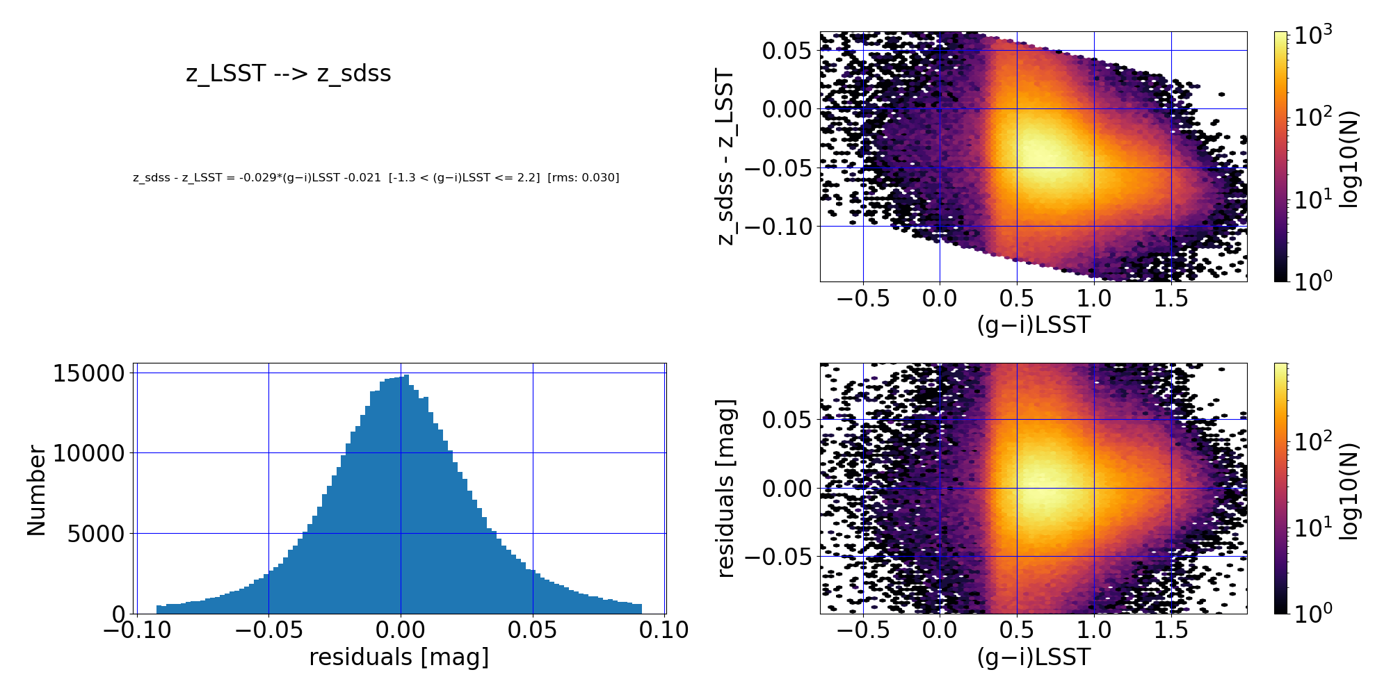
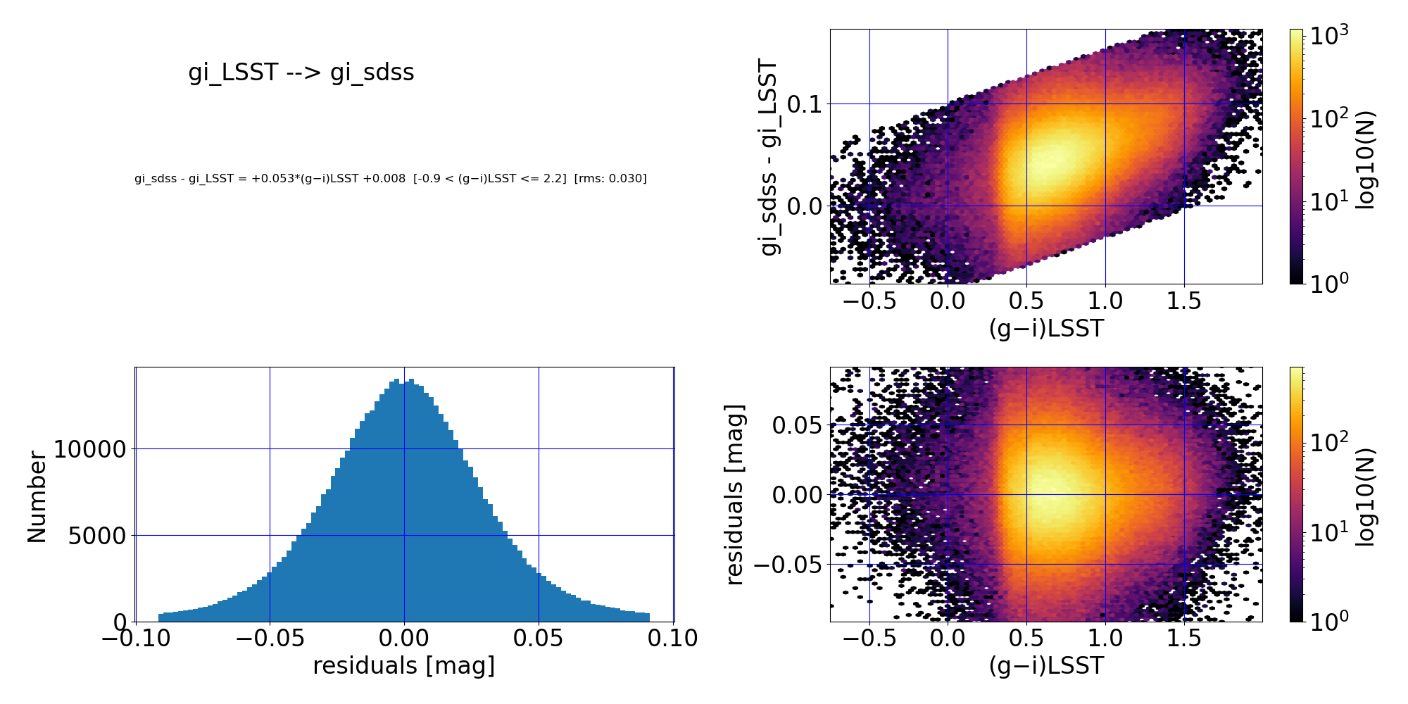
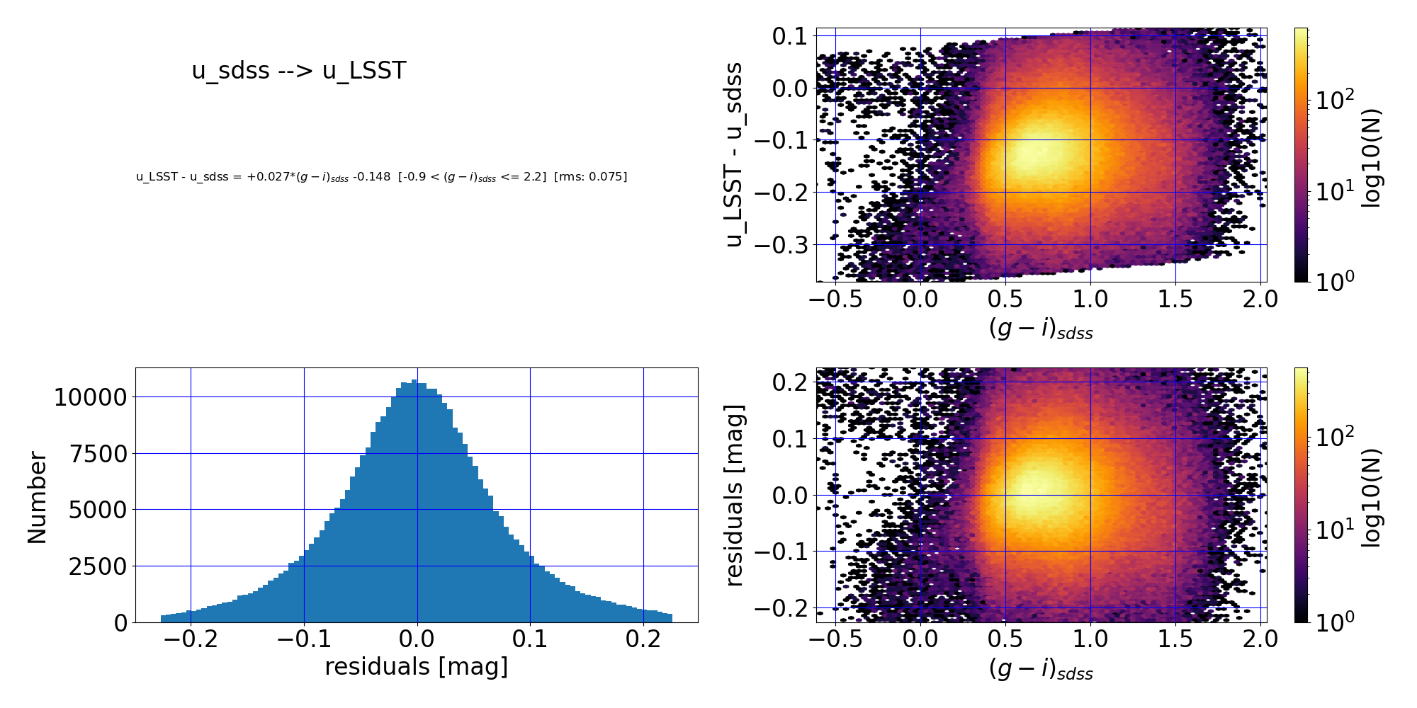
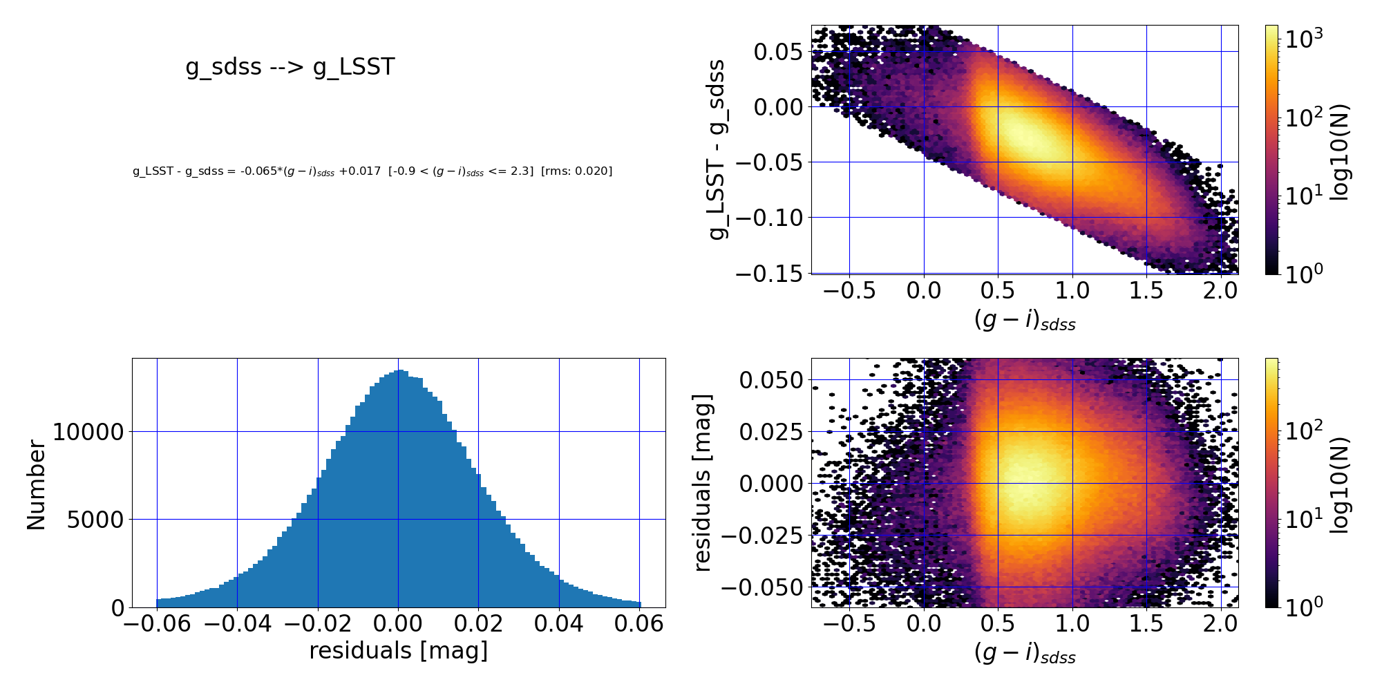
1.3.5 LSST DP2 <–> SDSS DR18#

Conversion	Transformation Equation	RMS	Applicable Color Range	QA Plot
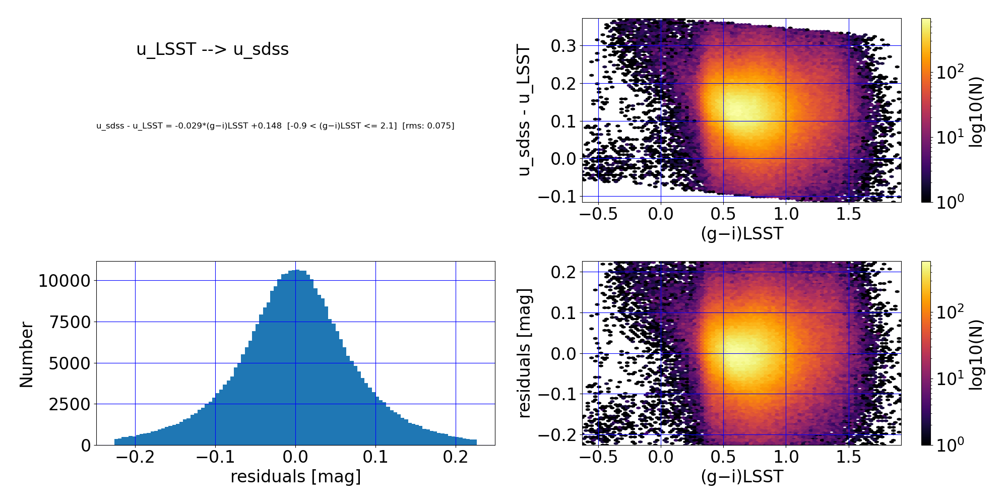
\(u_{LSST} \to u_{sdss}\)	\(u_{sdss} - u_{LSST} = -0.029 (g−i)LSST +0.148\)	0.075	\(-0.9 < (g−i)LSST \leq 2.1\)	link

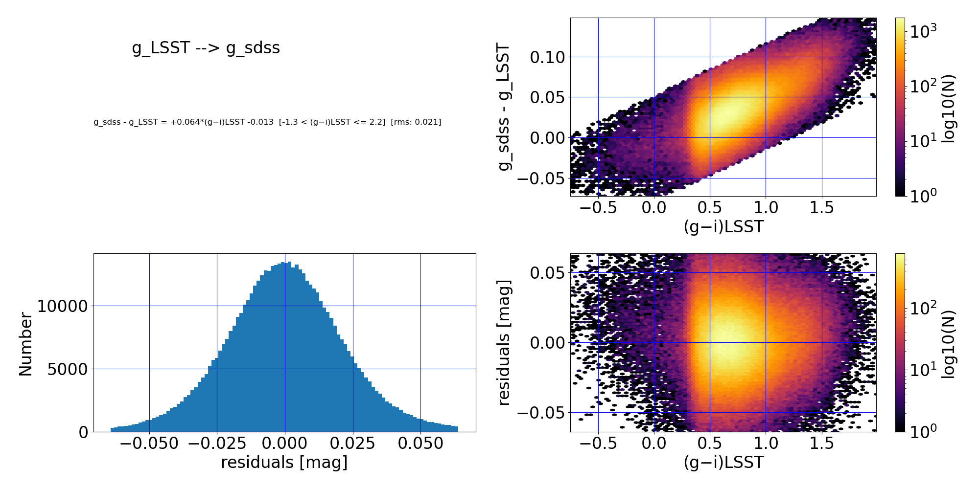
\(g_{LSST} \to g_{sdss}\)	\(g_{sdss} - g_{LSST} = +0.064 (g−i)LSST -0.013\)	0.021	\(-1.3 < (g−i)LSST \leq 2.2\)	link

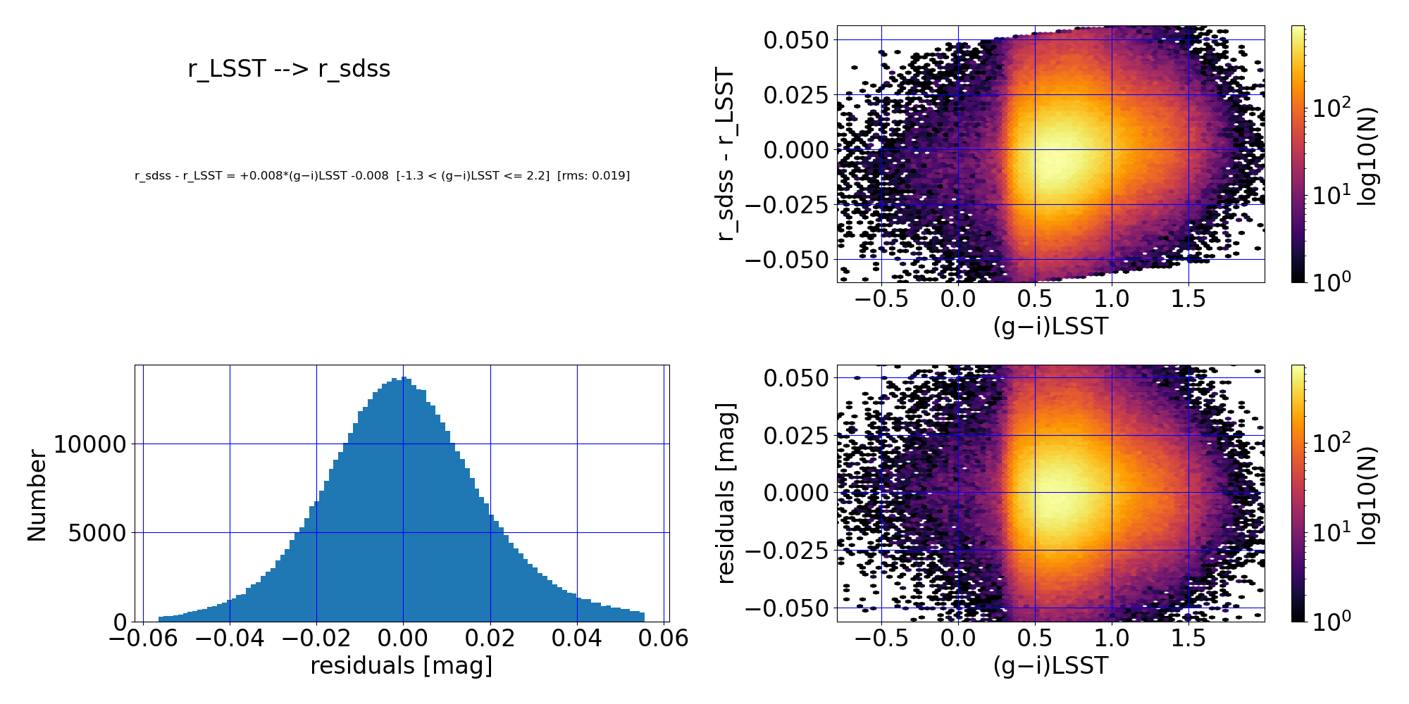
\(r_{LSST} \to r_{sdss}\)	\(r_{sdss} - r_{LSST} = +0.008 (g−i)LSST -0.008\)	0.019	\(-1.3 < (g−i)LSST \leq 2.2\)	link

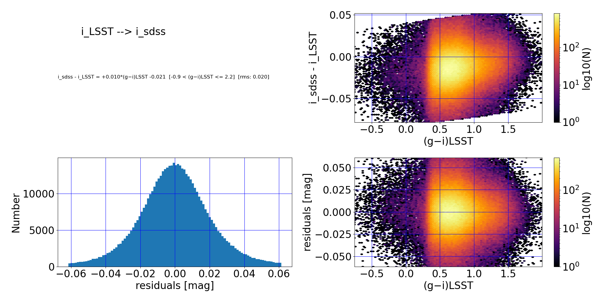
\(i_{LSST} \to i_{sdss}\)	\(i_{sdss} - i_{LSST} = +0.010 (g−i)LSST -0.021\)	0.02	\(-0.9 < (g−i)LSST \leq 2.2\)	link

\(z_{LSST} \to z_{sdss}\)	\(z_{sdss} - z_{LSST} = -0.029 (g−i)LSST -0.021\)	0.03	\(-1.3 < (g−i)LSST \leq 2.2\)	link

\(gi_{LSST} \to gi_{sdss}\)	\(gi_{sdss} - gi_{LSST} = +0.053 (g−i)LSST +0.008\)	0.03	\(-0.9 < (g−i)LSST \leq 2.2\)	link

Conversion	Transformation Equation	RMS	Applicable Color Range	QA Plot
\(u_{sdss} \to u_{LSST}\)	\(u_{LSST} - u_{sdss} = +0.027 (g-i)_{sdss} -0.148\)	0.075	\(-0.9 < (g-i)_{sdss} \leq 2.2\)	link

\(g_{sdss} \to g_{LSST}\)	\(g_{LSST} - g_{sdss} = -0.065 (g-i)_{sdss} +0.017\)	0.02	\(-0.9 < (g-i)_{sdss} \leq 2.3\)	link

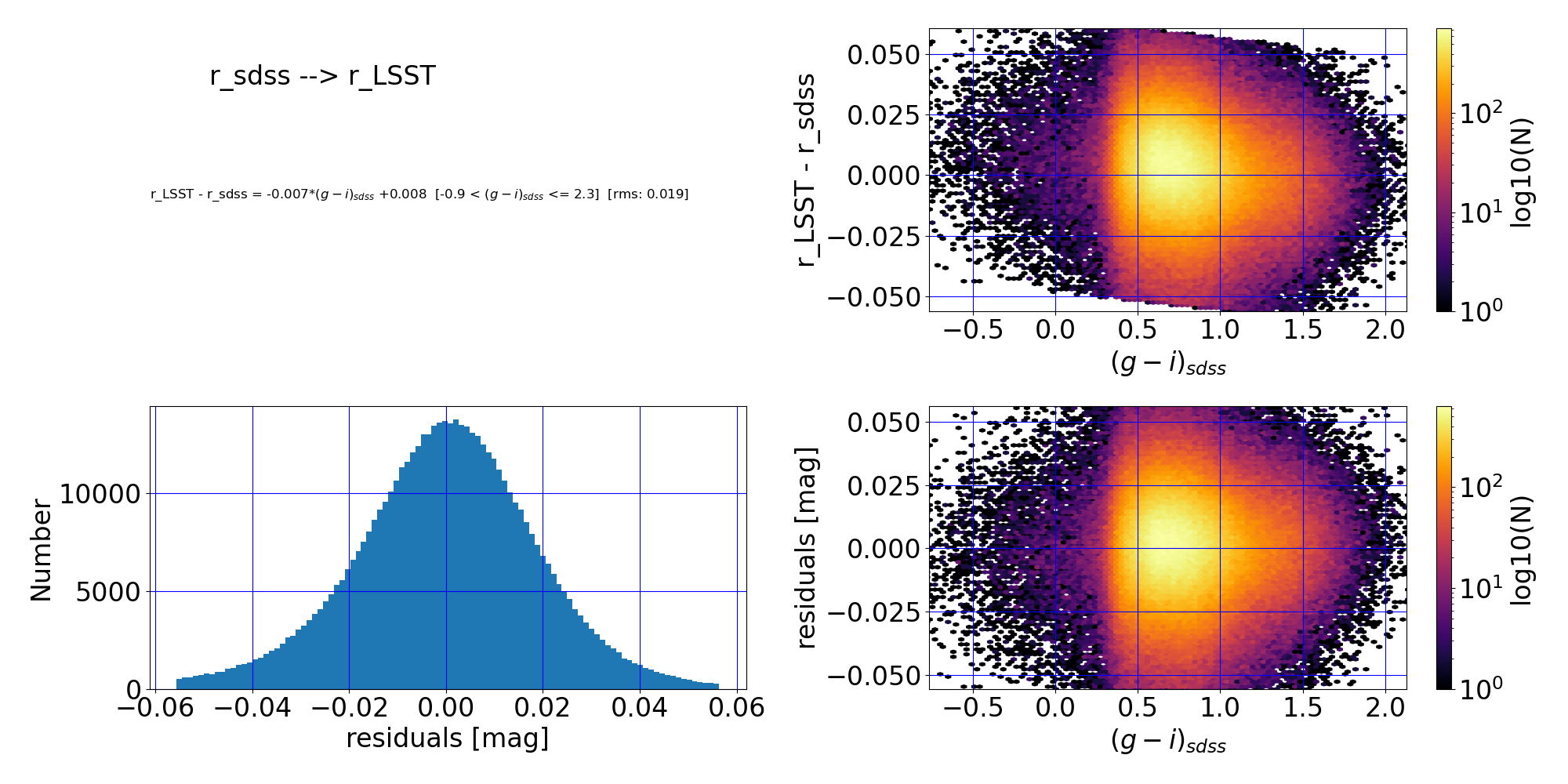
\(r_{sdss} \to r_{LSST}\)	\(r_{LSST} - r_{sdss} = -0.007 (g-i)_{sdss} +0.008\)	0.019	\(-0.9 < (g-i)_{sdss} \leq 2.3\)	link

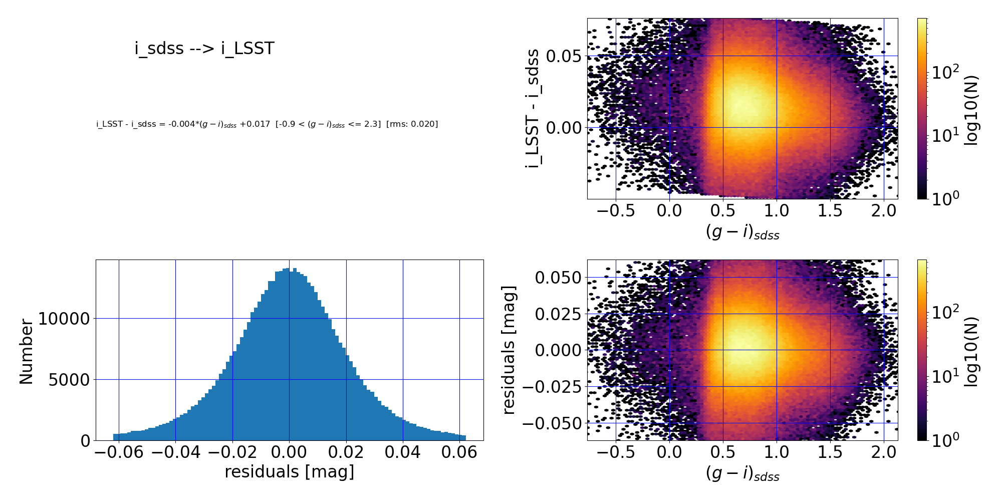
\(i_{sdss} \to i_{LSST}\)	\(i_{LSST} - i_{sdss} = -0.004 (g-i)_{sdss} +0.017\)	0.02	\(-0.9 < (g-i)_{sdss} \leq 2.3\)	link

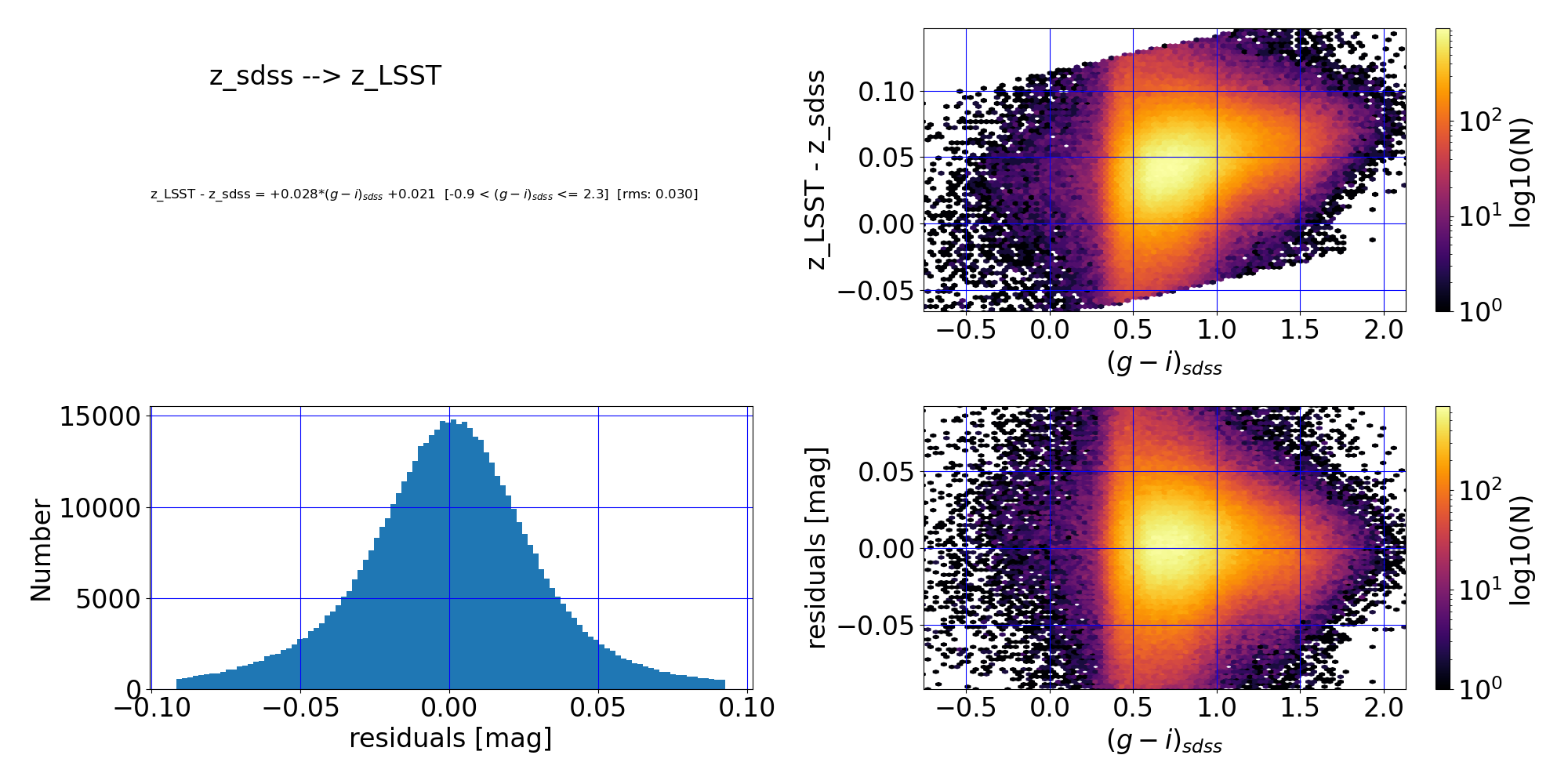
\(z_{sdss} \to z_{LSST}\)	\(z_{LSST} - z_{sdss} = +0.028 (g-i)_{sdss} +0.021\)	0.03	\(-0.9 < (g-i)_{sdss} \leq 2.3\)	link

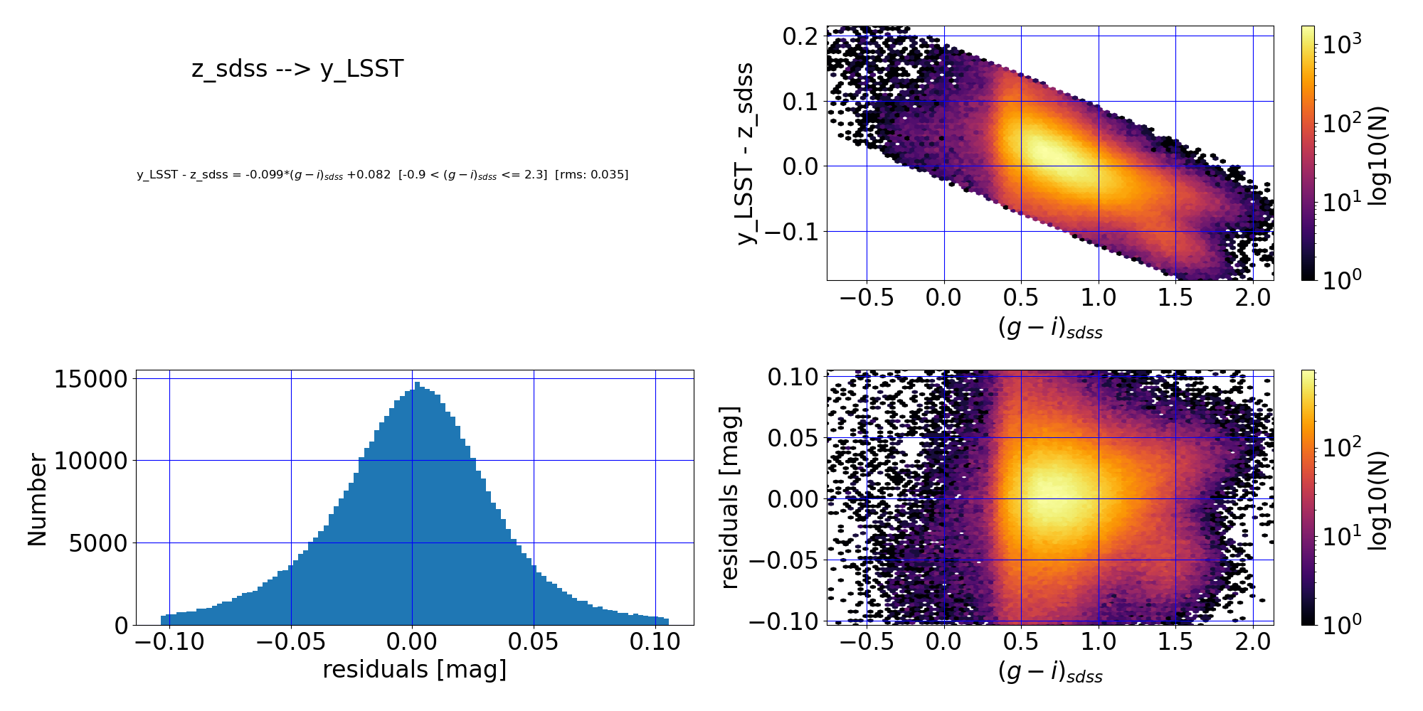
\(z_{sdss} \to y_{LSST}\)	\(y_{LSST} - z_{sdss} = -0.099 (g-i)_{sdss} +0.082\)	0.035	\(-0.9 < (g-i)_{sdss} \leq 2.3\)	link

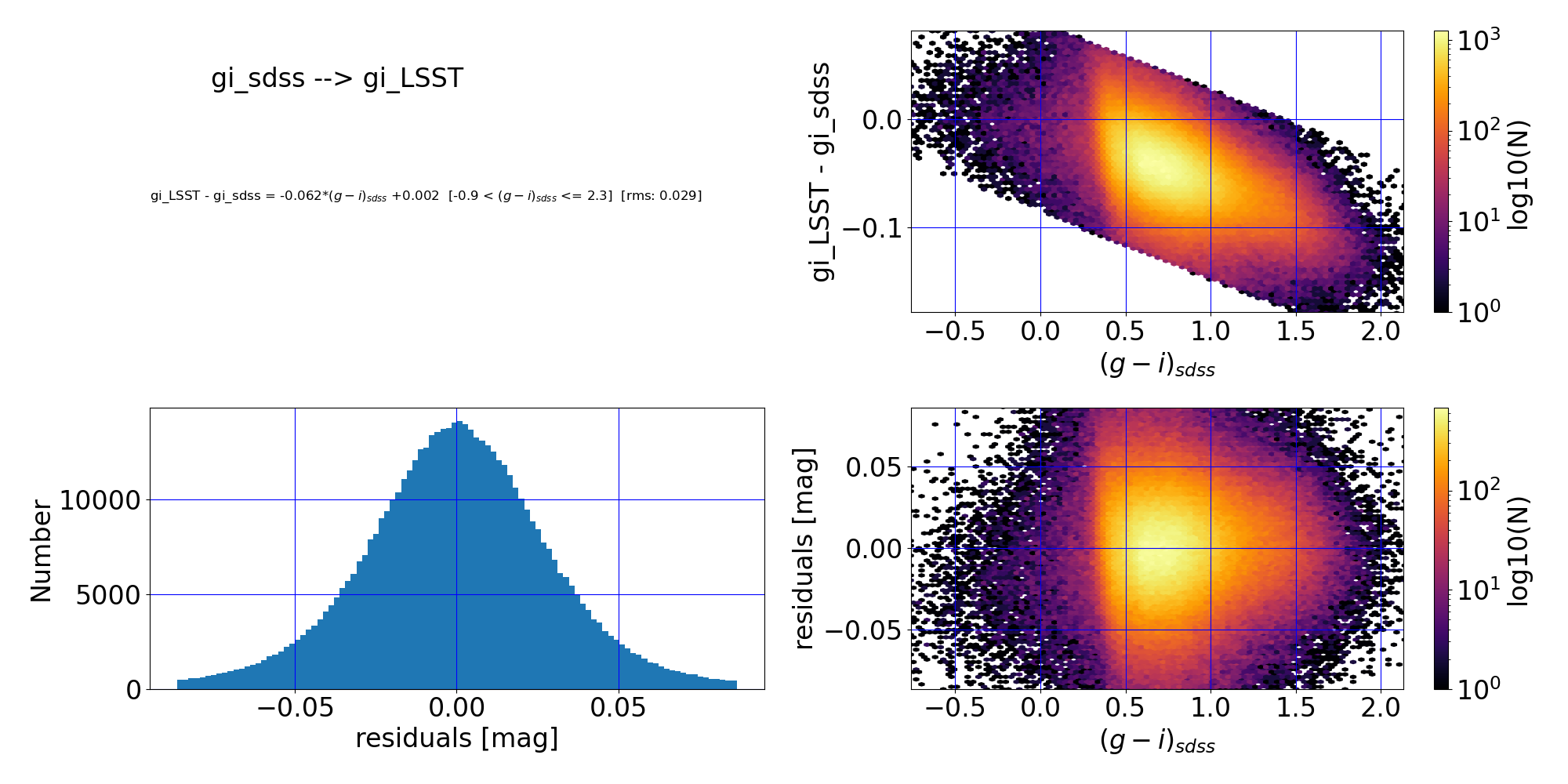
\(gi_{sdss} \to gi_{LSST}\)	\(gi_{LSST} - gi_{sdss} = -0.062 (g-i)_{sdss} +0.002\)	0.029	\(-0.9 < (g-i)_{sdss} \leq 2.3\)	link

1.3.6 LSST DP2 <–> Euclid#

Under Construction

1.3.7 LSST DP2 <–> Johnson-Cousins UBVRcIc#

Conversion	Transformation Equation	RMS	Applicable Color Range	QA Plot
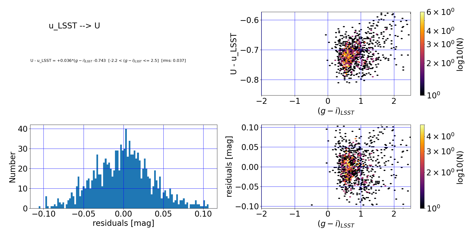
\(u_{LSST} \to U\)	\(U - u_{LSST} = +0.036 (g-i)_{LSST} -0.743\)	0.037	\(-2.2 < (g-i)_{LSST} \leq 2.5\)	link

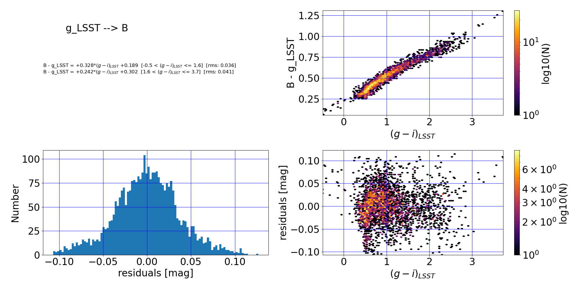
\(g_{LSST} \to B\)	\(B - g_{LSST} = +0.328 (g-i)_{LSST} +0.189\)	0.036	\(-0.5 < (g-i)_{LSST} \leq 1.6\)	link
\(g_{LSST} \to B\)	\(B - g_{LSST} = +0.242 (g-i)_{LSST} +0.302\)	0.041	\(1.6 < (g-i)_{LSST} \leq 3.7\)	link

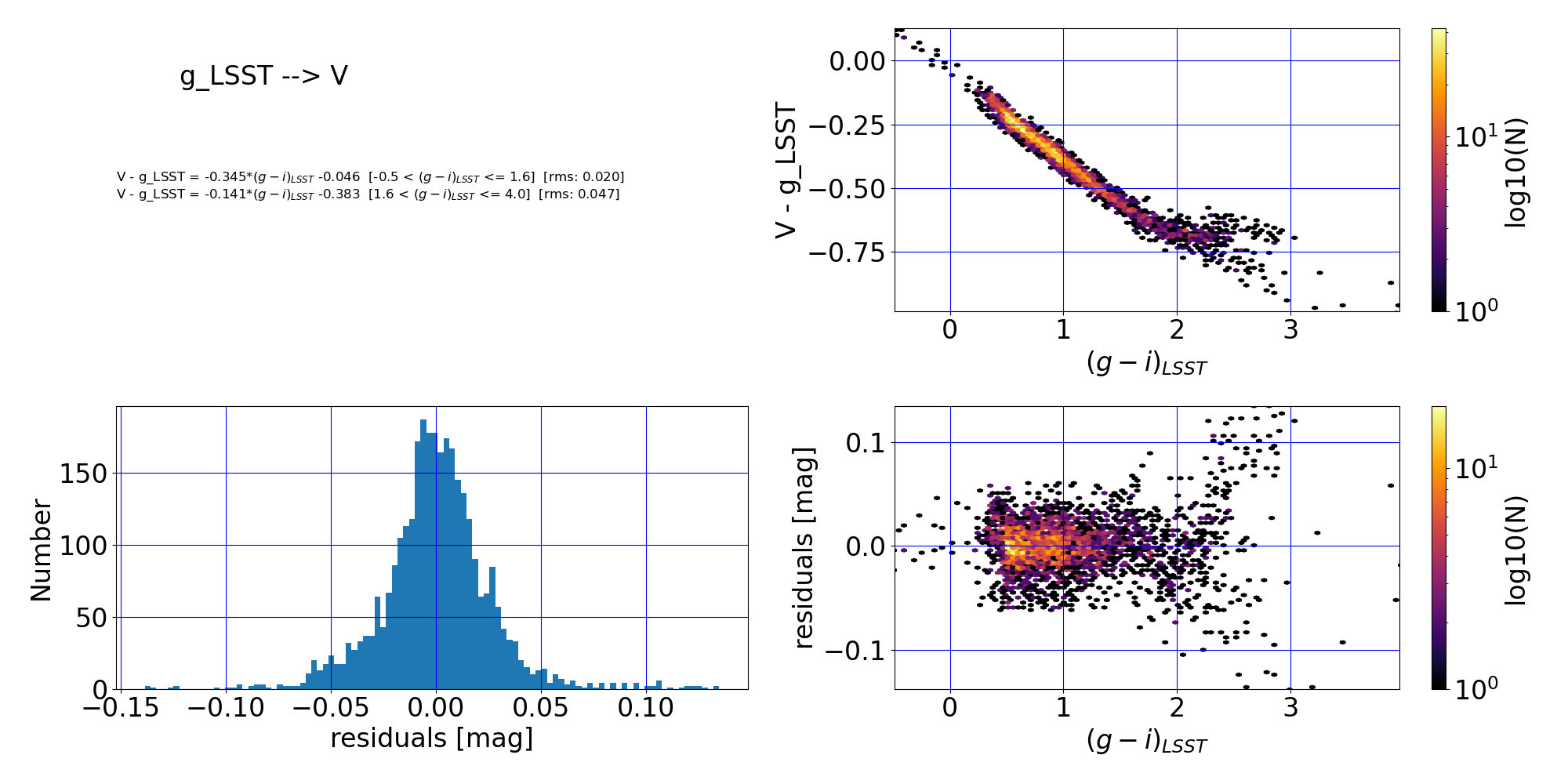
\(g_{LSST} \to V\)	\(V - g_{LSST} = -0.345 (g-i)_{LSST} -0.046\)	0.02	\(-0.5 < (g-i)_{LSST} \leq 1.6\)	link
\(g_{LSST} \to V\)	\(V - g_{LSST} = -0.141 (g-i)_{LSST} -0.383\)	0.047	\(1.6 < (g-i)_{LSST} \leq 4.0\)	link

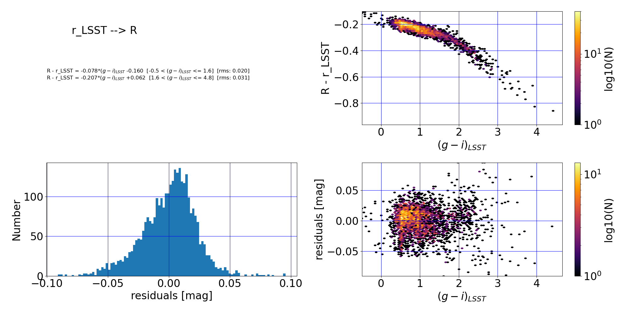
\(r_{LSST} \to R\)	\(R - r_{LSST} = -0.078 (g-i)_{LSST} -0.160\)	0.02	\(-0.5 < (g-i)_{LSST} \leq 1.6\)	link
\(r_{LSST} \to R\)	\(R - r_{LSST} = -0.207 (g-i)_{LSST} +0.062\)	0.031	\(1.6 < (g-i)_{LSST} \leq 4.8\)	link

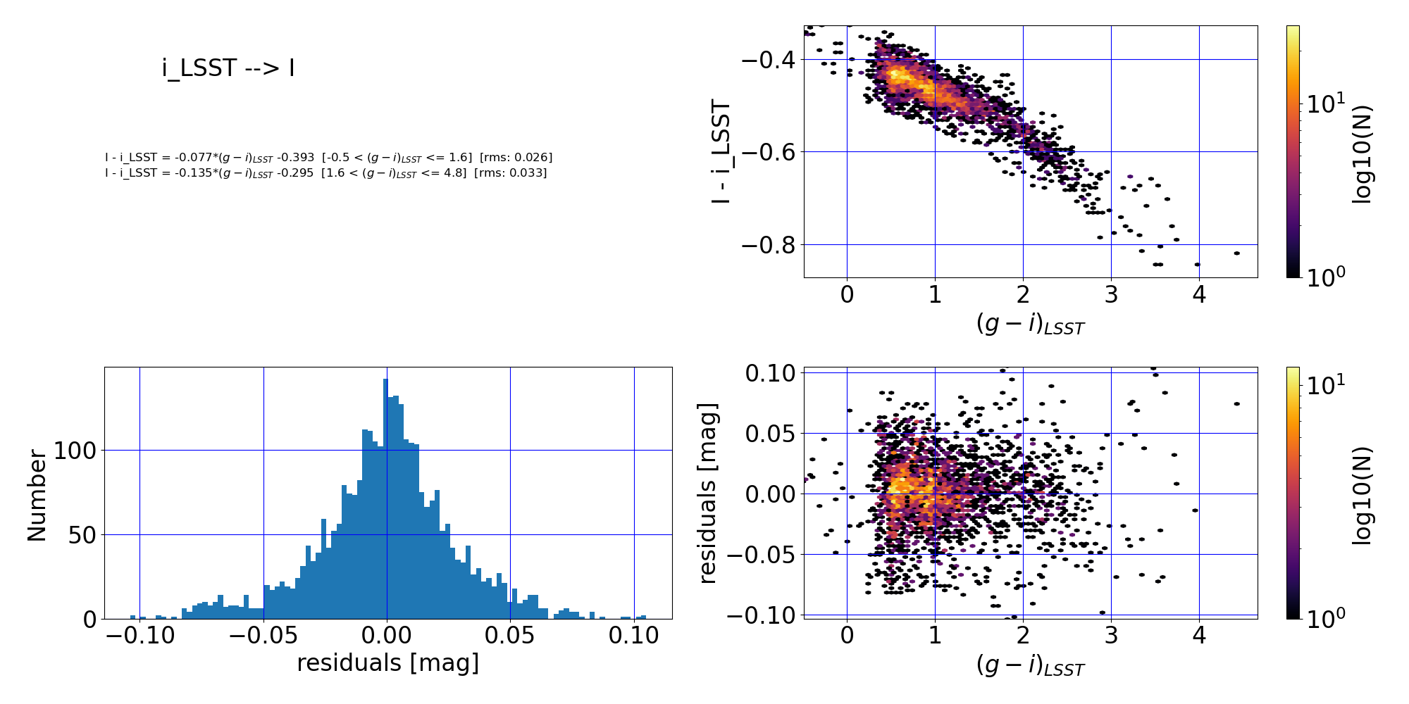
\(i_{LSST} \to I\)	\(I - i_{LSST} = -0.077 (g-i)_{LSST} -0.393\)	0.026	\(-0.5 < (g-i)_{LSST} \leq 1.6\)	link
\(i_{LSST} \to I\)	\(I - i_{LSST} = -0.135 (g-i)_{LSST} -0.295\)	0.033	\(1.6 < (g-i)_{LSST} \leq 4.8\)	link

Conversion	Transformation Equation	RMS	Applicable Color Range	QA Plot
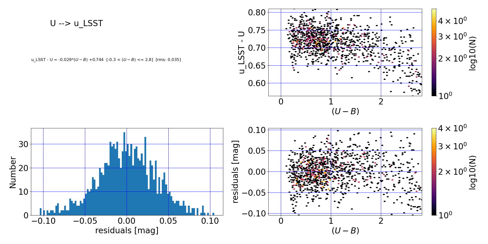
\(U \to u_{LSST}\)	\(u_{LSST} - U = -0.029 (U-B) +0.744\)	0.035	\(-0.3 < (U-B) \leq 2.8\)	link

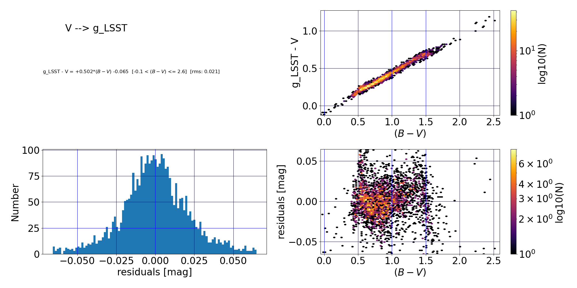
\(V \to g_{LSST}\)	\(g_{LSST} - V = +0.502 (B-V) -0.065\)	0.021	\(-0.1 < (B-V) \leq 2.6\)	link

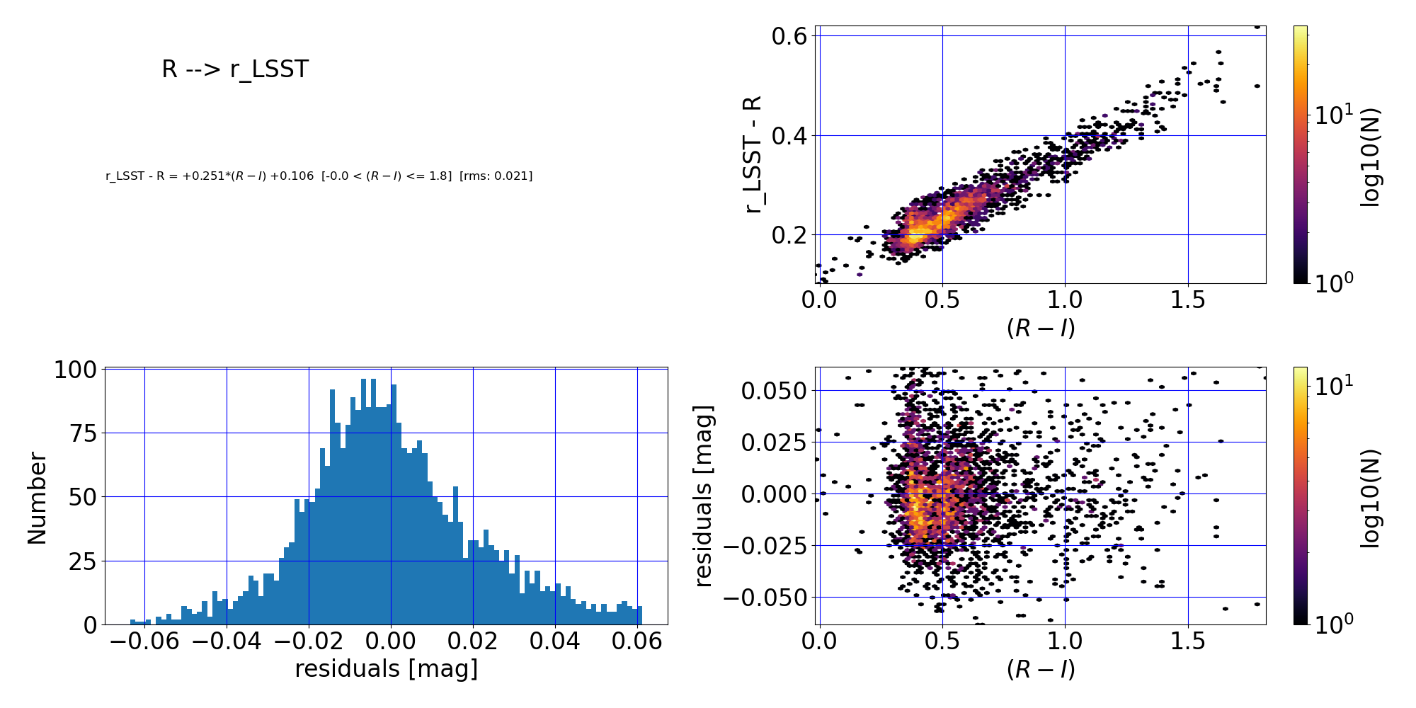
\(R \to r_{LSST}\)	\(r_{LSST} - R = +0.251 (R-I) +0.106\)	0.021	\(-0.0 < (R-I) \leq 1.8\)	link

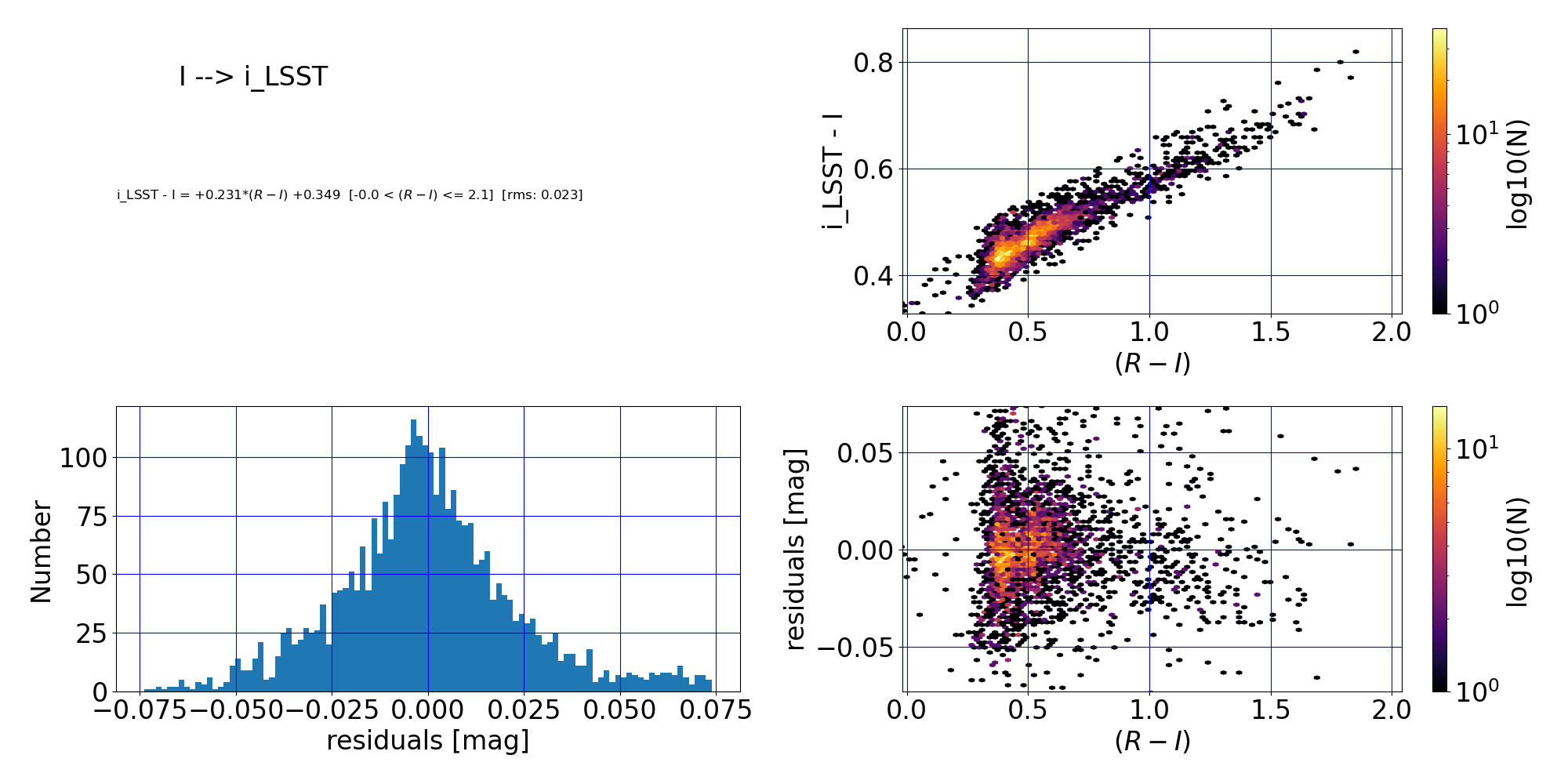
\(I \to i_{LSST}\)	\(i_{LSST} - I = +0.231 (R-I) +0.349\)	0.023	\(-0.0 < (R-I) \leq 2.1\)	link

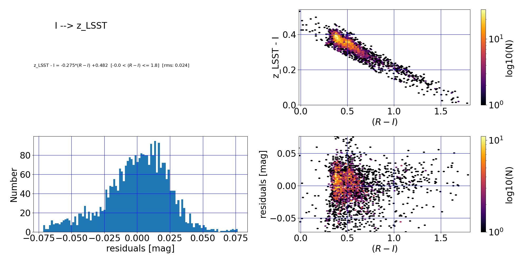
\(I \to z_{LSST}\)	\(z_{LSST} - I = -0.275 (R-I) +0.482\)	0.024	\(-0.0 < (R-I) \leq 1.8\)	link

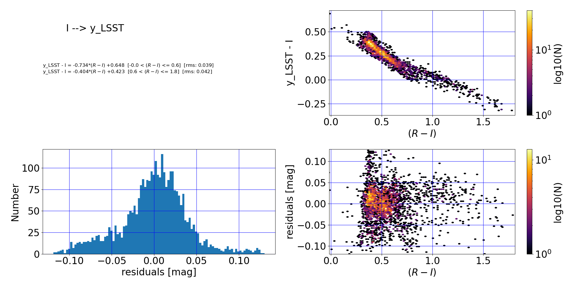
\(I \to y_{LSST}\)	\(y_{LSST} - I = -0.734 (R-I) +0.648\)	0.039	\(-0.0 < (R-I) \leq 0.6\)	link
\(I \to y_{LSST}\)	\(y_{LSST} - I = -0.404 (R-I) +0.423\)	0.042	\(0.6 < (R-I) \leq 1.8\)	link

2. Lookup Table (Interpolation) Transformations#

2.1. Overview#

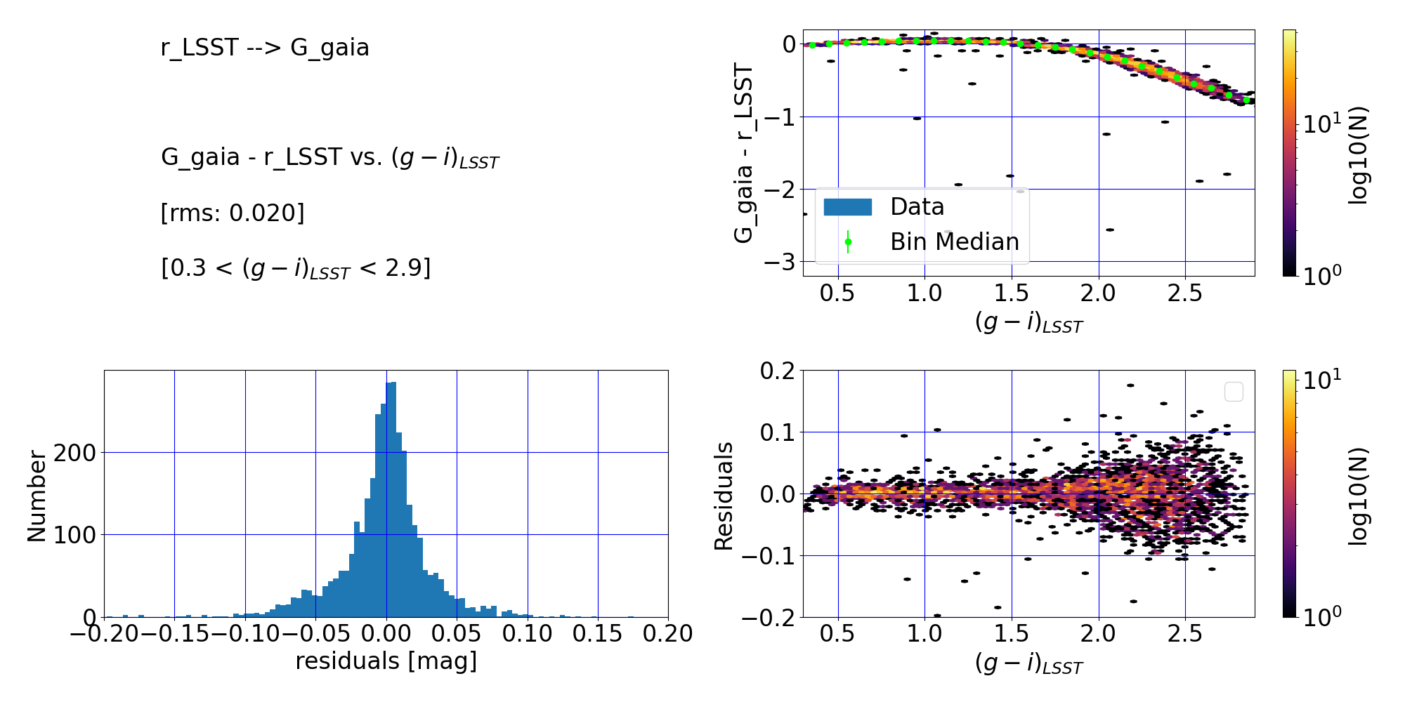
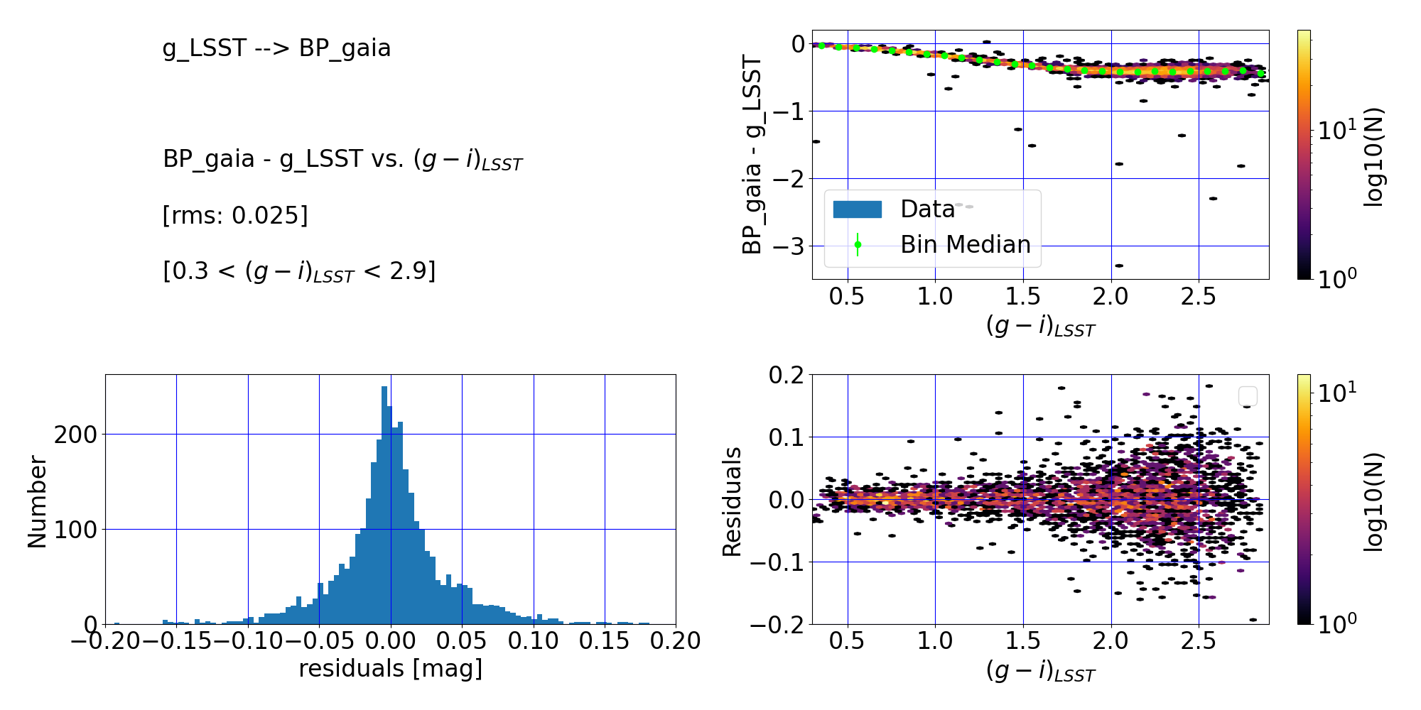
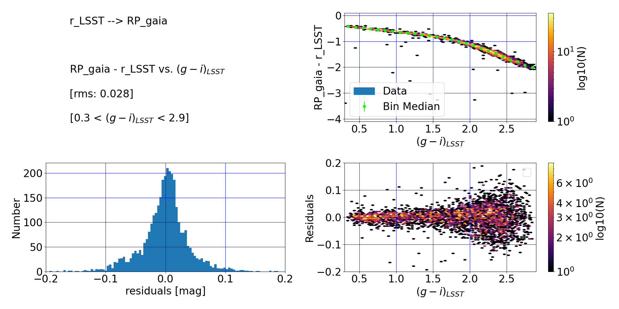
Interpolation methods were used to model complex or non-linear relationships between survey measurements. These methods rely on binning color indices and computing median magnitude differences.

The lookup tables included in the tables below can be used to convert data from one photometric system to the other via interpolation methods. The files contain the delta_mag vs color locus in bins of (typically) 0.1-mag binsize along the color axis. Here is a python code that takes the lookup table CSV file for the transformation from LSST DP2 \(g\)-band and \((g-i)\) color to DES \(g\)-band. The code makes use of the scipy interpolate routine.

import pandas as pd
from scipy import interpolate

# Read in lookup table CSV file...
lut_name = 'transInterp.ComCam_to_des.g_gi_ComCam.csv'
df_interp = pd.read_csv(lut_name)

# Create linear interpolation of the median dmag vs. color
#  bin calculated above...
response = interpolate.interp1d(\
                  df_interp.bin_label.values.astype(float), \
                  df_interp.bin_median.values, \
                  bounds_error=False, fill_value=0., \
                  kind='linear')

# Read in file with data to be transformed...
df = pd.read_csv(inputFile)
# The following assumes a column with LSST DP2 g and
# a column with LSST DP2 (g-i) in this file...
df['offset'] = response(df['gi_ComCam'].values)
df['g_des'] = df['g_ComCam'] + df['offset']

2.2 LSST DP2 Transformations#

2.2.1 LSST DP2 <–> DES DR2#

Under Construction

2.2.2 LSST DP2 <–> Panstarrs1 DR2#

Under Construction

2.2.3 LSST DP2 <–> GAIA DR3#

Conversion	RMS	Applicable Color Range	QA Plot	Lookup Table
\(r_{LSST} \to G_{gaia}\)	0.02	\(0.3 < (g-i)_{LSST} < 2.9\)	link	link
\(g_{LSST} \to BP_{gaia}\)	0.025	\(0.3 < (g-i)_{LSST} < 2.9\)	link	link
\(r_{LSST} \to RP_{gaia}\)	0.028	\(0.3 < (g-i)_{LSST} < 2.9\)	link	link

Conversion	RMS	Applicable Color Range	QA Plot	Lookup Table
\(G_{gaia} \to g_{LSST}\)	0.027	\(0.6 < (BP-RP)_{gaia} < 2.9\)	link	link
\(G_{gaia} \to r_{LSST}\)	0.018	\(0.6 < (BP-RP)_{gaia} < 2.9\)	link	link
\(G_{gaia} \to i_{LSST}\)	0.01	\(0.6 < (BP-RP)_{gaia} < 2.9\)	link	link
\(G_{gaia} \to z_{LSST}\)	0.018	\(0.6 < (BP-RP)_{gaia} < 2.9\)	link	link
\(G_{gaia} \to y_{LSST}\)	0.024	\(0.6 < (BP-RP)_{gaia} < 2.9\)	link	link

2.2.4 LSST DP2 <–> SDSS DR18#

Under Construction

2.2.5 LSST DP2 <–> Euclid#

Under Construction

2.2.6 LSST DP2 <–> Stetson UBVRcIc#

Under Construction

References#

[1]

Meagan N. Porter, Douglas L. Tucker, J. Allyn Smith, and Christina L. Adair. Photometric Transformation Relations for the LSST Data Preview 1. Technical Note RTN-099, NSF-DOE Vera C. Rubin Observatory, July 2026. URL: https://rtn-099.lsst.io/, doi:10.71929/rubin/3006074.

[2]

NSF-DOE Vera C. Rubin Observatory. Legacy Survey of Space and Time Data Preview 2 [Data set]. 2026. URL: https://www.osti.gov//servlets/purl/3382528, doi:10.71929/rubin/3382528.

[3]

A. J. Pickles. A Stellar Spectral Flux Library: 1150-25000 Å. PASP, 110(749):863–878, July 1998. doi:10.1086/316197.

[4]

SLAC National Accelerator Laboratory and NSF-DOE Vera C. Rubin Observatory. LSST Commissioning Camera. 2024. URL: https://www.osti.gov//servlets/purl/2561361, doi:10.71929/RUBIN/2561361.

[5]

SLAC National Accelerator Laboratory and NSF-DOE Vera C. Rubin Observatory. The LSST Camera (LSSTCam). 2025. URL: https://www.osti.gov//servlets/purl/2571927, doi:10.71929/rubin/2571927.

[6]

Vera C. Rubin Observatory Team. The Vera C. Rubin Observatory Data Preview 1. Technical Note RTN-095, NSF-DOE Vera C. Rubin Observatory, May 2026. URL: https://rtn-095.lsst.io/, doi:10.71929/rubin/2570536.

[7]

Vera C. Rubin Observatory Team. The Vera C. Rubin Observatory Data Preview 2. Technical Note RTN-115, NSF-DOE Vera C. Rubin Observatory, July 2026. URL: https://rtn-115.lsst.io/, doi:10.71929/rubin/3377440.

[8]

Vera C. Rubin Observatory Team, Tatiana Acero-Cuellar, Emily Acosta, and others. The Vera C. Rubin Observatory Data Preview 1. AJ, 171(6):360, June 2026. arXiv:2603.23786, doi:10.3847/1538-3881/ae521f.

Version

Source

Photometric Transformation Relations for the LSST Data Preview 2#

Abstract

0. General Overview#

1. Polynomial Fit Transformations#

1.1. Overview#

1.2. Synthetic LSSTCam Transformations#

1.2.1 LSST <–> TESS#

1.3. Observed LSST DP2 Transformations#

1.3.1 LSST DP2 <–> LSST DP1#

1.3.2 LSST DP2 <–> DES DR2#

1.3.3 LSST DP2 <–> PanStarrs1 DR2#

1.3.4 LSST DP2 <–> GAIA DR3#

1.3.5 LSST DP2 <–> SDSS DR18#

1.3.6 LSST DP2 <–> Euclid#

1.3.7 LSST DP2 <–> Johnson-Cousins UBVRcIc#

2. Lookup Table (Interpolation) Transformations#

2.1. Overview#

2.2 LSST DP2 Transformations#

2.2.1 LSST DP2 <–> DES DR2#

2.2.2 LSST DP2 <–> Panstarrs1 DR2#

2.2.3 LSST DP2 <–> GAIA DR3#

2.2.4 LSST DP2 <–> SDSS DR18#

2.2.5 LSST DP2 <–> Euclid#

2.2.6 LSST DP2 <–> Stetson UBVRcIc#

References#